How we build the portfolio

Dear investors,

In the past two letters, we discussed how we identify investment opportunities and how we assess the risks associated with each of them. In this letter, we address the final step: how we combine these individual opportunities into a coherent investment portfolio for our funds.

Our objective is to allocate capital to the best opportunities available at any given time, while avoiding excessive exposure to downside risk. Approved investment theses must be compared against one another to determine appropriate position sizing, which requires a consistent framework for evaluation. At the same time, we must manage portfolio-level risk, which emerges from the combination of selected positions and their respective allocations. Below, we explain how we approach these challenges.

How We Compare Investment Theses

In theory, comparing investment theses is straightforward: one simply evaluates their expected returns relative to their respective levels of risk. The thesis offering the highest return per unit of risk is the most attractive. In practice, however, there is no precise or objective method for measuring these two variables with accuracy.

For each investment thesis, we build a financial model that simulates the company’s future performance and allows us to estimate its value by discounting expected cash flows. Because this model depends on a range of uncertain assumptions, the resulting valuation is inherently uncertain as well. Referring to a single “fair value” is a conventional simplification. A more realistic perspective is that there exists a range of possible intrinsic values, depending on how future outcomes unfold. By running multiple simulations and varying the most relevant assumptions, we can derive a distribution of potential values similar to the one illustrated below.

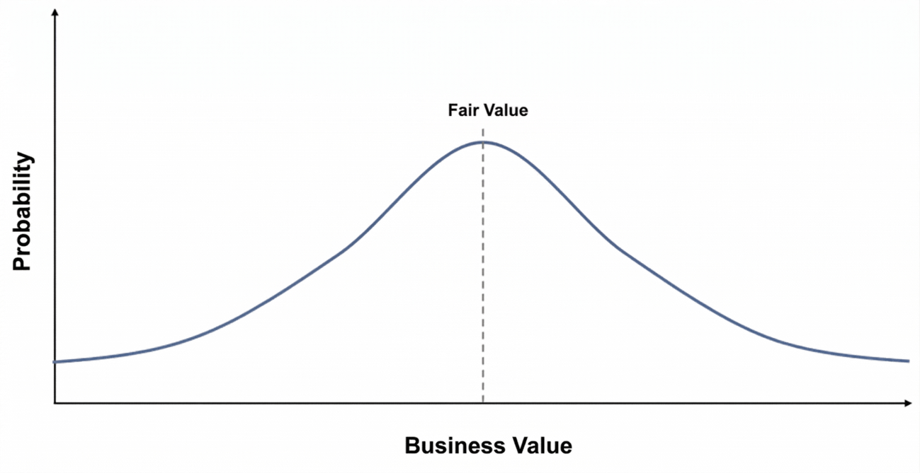
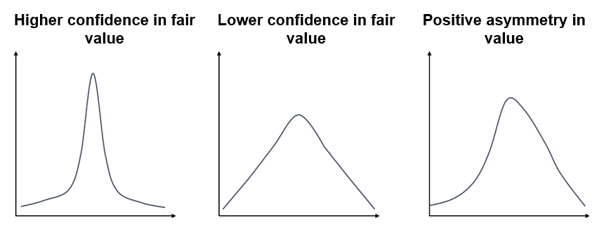
What we refer to as “fair value” is the mean of this probability distribution—but this is not the only relevant information. The shape of the distribution also matters. Narrow distributions indicate more stable business and greater confidence in projections, while wider distributions imply higher uncertainty and risk. In some cases, the distribution may be asymmetric, with a skew toward either upside or downside outcomes.

We simplify these results for practical use as follows: what matters most is the range of most likely outcomes, so we can exclude the “tails” of the distribution and focus on the interval that represents roughly 90% of the probability mass. Instead of relying solely on the mean as a reference, we track three key points: the mean, the lower bound, and the upper bound. This allows us to assess the risk–return profile of each investment thesis by comparing the market price to these reference points. The discount of the market price relative to the mean is what we refer to as the margin of safety. Meanwhile, the ratio between potential upside and downside is defined as the difference between the price and the upper bound divided by the difference between the price and the lower bound, as illustrated below.

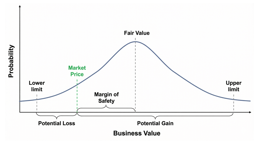
With these analyses in place, comparing investment theses once again becomes straightforward. The higher the margin of safety and the greater the ratio between potential upside and downside, the more attractive the thesis.

Alongside this quantitative framework, we also assess qualitative aspects of each company based on a predefined set of criteria—for example, the level of competitiveness within its industry, the strength of its competitive advantages, exposure to different risk factors, growth potential, and so on. Each factor is assigned a score on a standardized scale, and the combination of these individual scores results in an overall rating that reflects our view of the business’s quality. This methodology, commonly referred to as a scorecard, allows us to compare factors that are difficult to quantify directly but remain relevant for capital allocation decisions.

By combining the quantitative metrics with the qualitative scorecard, we rank approved investment theses according to their overall attractiveness and form an initial view of which positions should receive higher or lower capital allocation. Additional steps are then required to determine the final portfolio weights for each thesis.

Position Size Limits

Two factors constrain the size of any individual position in our portfolio. The first is liquidity. We must ensure that our funds are able to return capital to investors upon request, so each investment is capped at a size that can still be liquidated within the fund’s redemption period. The second is the downside risk embedded in the thesis, regardless of its upside potential.

Consider an investment that could result in an 80% loss in an adverse scenario but, on the other hand, could increase tenfold. The risk–reward profile is highly attractive, but allocating a large portion of the portfolio to such a position would not be prudent given the magnitude of the potential loss. As a practical rule, we define the maximum percentage of the portfolio we are willing to expose to the downside risk of a given thesis and size the position accordingly. For example, if this limit is 4%, the hypothetical investment above could receive a maximum allocation of 5% (5% × 80% = 4%). If the potential loss were 25%, the maximum allocation would be 16%.

These limits—particularly the cap on portfolio exposure to a single thesis—make it necessary to allocate capital across multiple positions. This is the well-known principle of diversification, often advocated as a way to mitigate investment risk.

Effective Diversification

The rationale for diversification is easy to understand through a simple analogy with repeated dice rolls. In just five rolls, it is difficult to predict how many times a six will appear. In 6,000 rolls, however, it is highly likely that a six will occur approximately 1,000 times. This reflects a statistical principle known as the Law of Large Numbers: the larger the sample size, the more stable and predictable the average outcome becomes.

The logic behind diversification in investing is analogous. If we hold multiple investment opportunities with uncorrelated returns, the realized portfolio return should converge toward the expected return derived from each thesis (assuming the estimates are correct). The key point, however, is that investment theses are not repeatable events like dice rolls, and the existence of a large number of opportunities with similar risk–return profiles is a purely theoretical construct. In practice, truly attractive opportunities are scarce, and their quality declines quickly as we move down the ranking. In other words, the tenth-best idea is already meaningfully worse than the first. For this reason, it is necessary to strike a balance between sufficient diversification to manage risk and adequate concentration in the best ideas to achieve attractive returns.

We typically hold between 5 and 15 positions in the portfolio, depending on the number of sufficiently attractive opportunities available at a given time. During market downturns, it is easier to find multiple viable investments, allowing for greater diversification. In strong markets, opportunities become scarcer, and the portfolio tends to be more concentrated.

Our target number of positions is relatively small compared to common market practice, but this is a deliberate choice. The marginal benefit of diversification declines as more positions are added, while the quality of incremental ideas tends to deteriorate. Beyond a certain point, adding a new position can actually increase portfolio risk—even after accounting for diversification benefits—due to the lower quality of the additional investment.

Because our portfolio is concentrated on the best investment theses, we need to ensure that they are not strongly correlated with each other, in order to keep the risk level under control. It's not enough to assess whether the companies are in different economic sectors. We map which variables have a significant impact on each thesis and take care not to concentrate the portfolio on companies that are heavily dependent on the same economic variables. To illustrate, imagine a city entirely focused on tourism. If you invest in a gas station, a restaurant, a hotel, and a clothing store, all your businesses will still be highly dependent on the same factor: the number of people who will visit that city during the season. Because our portfolio is concentrated in our best ideas, we must ensure that these positions are not highly correlated with one another in order to keep overall risk under control. It is not sufficient to assess whether companies operate in different industries. Instead, we identify the key variables that materially impact each thesis and avoid concentrating the portfolio in businesses that are heavily exposed to the same underlying drivers.

As a simple illustration, consider a city heavily dependent on tourism. If you invest in a gas station, a restaurant, a hotel, and a clothing store, all of these businesses would still depend on a single factor: the number of visitors to the city during the season. With the list of approved theses ranked by attractiveness, their individual position limits defined, and a clear understanding of their underlying correlations, we can determine how much capital to allocate to each opportunity. This allocation process is dynamic. As market prices evolve and businesses themselves change over time, the portfolio must be periodically reassessed.

Monitoring and Rebalancing

If we assumed that our valuation estimates were precise, it would make sense to rebalance the portfolio frequently—even in response to small price fluctuations of just a few percentage points. In reality, however, investing is far from a precise activity. Valuation estimates are inherently rough, and price movements contain significant noise. Excessively frequent rebalancing would therefore increase transaction costs and consume team resources without a meaningful likelihood of improving overall returns.

We continuously monitor new information relevant to our existing positions, but we only rebalance the portfolio when there are material changes in expectations for one or more companies, or when there are significant movements in their market prices. To prevent this approach from becoming complacent, we periodically conduct a full portfolio review—comparing all current positions against one another, as well as against investment theses that were approved but not included in the portfolio due to valuation or correlation constraints. This exercise is akin to rebuilding the portfolio from scratch and helps ensure that current allocations reflect deliberate, rational decisions rather than inertia.

Even with all these precautions, every investor knows that it is impossible to consistently time the exact moments to buy and sell each stock. Trading near absolute tops or bottoms depends far more on luck than on skill. Our objective is to buy and sell within price ranges where these decisions are well justified. By applying this discipline consistently over the past decade, we have delivered attractive returns for our investors—and we expect this approach to continue generating strong results over time.